Conditional Formatting with Excel

Conditionally Formatting in Microsoft Excel is a useful tool, particularly as a student or business manager. Conditional formatting allows you to set a range of options on your data, such as sales target levels, assessments, results and much more. With conditional formatting, you can set figures or types of figures to appear against a coloured background, for example, if you wish to see a percentage of attendance for a group of students and see how the majority of the class is fairing, conditional formatting will allow you to set rules.

For example – class attendance figures:

Student Name	Attendance Rate	Observation Percent	Portfolio Percent
	71.43%	90.32%	27.27%
	0.00%	0.00%	0.00%
	71.43%	90.32%	27.27%
	42.86%	67.74%	18.18%
	71.43%	90.32%	27.27%
	71.43%	90.32%	27.27%
	71.43%	90.32%	27.27%
	57.14%	70.97%	27.27%
	28.57%	41.94%	18.18%
	42.86%	51.61%	9.09%

Looks rather plain, bland and boring, doesn’t it?

Define Your Rules

Now, let’s define the rules for our conditional formatting. Say we require a minimum of 50% attendance rate, and we want anything to be 49% and below to show as red. With an attendance rate of 80% or higher to be our optimum – we can set Excel to display this optimum range in green and the bits in-between (from 51-79%) can show as yellow – almost but not quite there.

-50%	Will appear like this
51%-79%	Will appear like this
80%+	Will appear like this

Set out your Spreadsheet

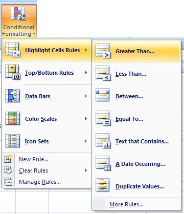
Start Excel and set out your spreadsheet. Select the rows you wish for the conditional formatting to apply. Click the CONDITIONAL FORMATTING button on the Home tab in the ribbon.

Set the Less than Option

Use the drop down arrow to select the options you wish to apply. In this example, set the first option to highlight all cells whose data is 50% or less. Choose the first option HIGHLIGHT CELLS RULES.

Follow the arrow across and choose the LESS THAN option. A dialogue box will appear for you to further set your options. You can either type the result you want, or use the select box to select a cell with the required data. The LIGHT RED FILL WITH DARK RED TEXT is set for us by default.

Click the OK button to set this option and return to your spreadsheet.

Set the Greater than Option

The cells in your spreadsheet should still be selected,  you can just continue setting your conditional formatting options. Click the CONDITIONAL FORMATTING button again, and this time select the HIGHLIGHT CELL RULES and then GREATER THAN.

Once more the dialogue box will appear on your screen. Again you can select the cell containing the data required, or you can type it directly into the box.

Use the drop down arrow to select the GREEN FILL WITH DARK GREEN TEXT which is the third default setting. Then click OK to return to your spreadsheet.

Set the between option

Finally, set the option to highlight the in-between numbers to yellow. With the cells in the spreadsheet still selected, click the CONDITIONAL FORMATTING button. Select the HIGHLIGHT CELL RULES and then across to BETWEEN.

In the dialogue box that pops up, set your additional options. Click the drop down arrow and choose the second option YELLOW FILL WITH DARK YELLOW TEXT. Click OK to return to your spreadsheet.

Completed Conditional Formatting

There you have a conditionally formatted spreadsheet. Try playing around with the figures and the colour scheme should automatically update for you.

Custom Formatting

Excel also allows you to set your own style of conditional formatting options. When setting your rules, you can choose CUSTOM style for fill and text combinations.

Have a play around with conditional formatting, it is a great tool to be able to use.